5. Bayesian regression

Mathematical modeling refers to the construction of mathematical expressions that describe the behavior of a variable of interest \(Y\). Frequently, we want to add to the model other variables (features) \(X\), which have information about the variable of interest \(Y\). This problem is known as regression. Formally, we look for a function \(f:\mathcal{X}\to\mathcal{Y}\) such that \(f(X)\) is a good approximation of \(Y\).

5.1. Bayesian linear regression, the Normal - Inverse-\(\chi^2\) model

Consider the usual regression model

\[Y=X^T\beta+\varepsilon,\]

with \(\varepsilon|X\sim \textsf{Normal}(0,\sigma^2)\) and \(\varepsilon\perp\!\!\!\perp\beta|X\).

And assume that we have a sample \(\mathcal{D}_n=\left((X_1,Y_1),\ldots,(X_n,Y_n)\right)\) with \((X_i,Y_i)\overset{iid}{\sim}(X,Y)\). Thus, the model can be written as

\[\mathbf{Y}=\mathbf{X}\beta+\vec{\varepsilon},\quad \vec{\varepsilon}\sim\textsf{Normal}_n(0,\sigma^2 I).\]

The parameters of this model are \(\beta\) and \(\sigma\).

See also

The accounts needed to deduce all the different distributions of the model presented in this chapter are extremely tedious, so I will limit myself to present here the results. Those interested readers can find in these notes all the details.

5.1.1. Prior distributions

Consider the following priors for this model

\[\begin{split} \begin{align*} \sigma^2 &\sim \textsf{Inverse-}\chi^2(\nu_0,\sigma_0^2),\quad \nu_0,\sigma_0>0, \\ \beta|\sigma^2 &\sim \textsf{Normal}_p(\mu_0, \sigma^2 V_0), \end{align*} \end{split}\]

with \(\mu_0\in \mathbb{R}^p\) and \(V_0\) a symmetric, positive definite matrix.

In this case we say that the joint distribution of \(\beta,\sigma^2\) is a Normal - Inverse-\(\chi^2\) distribution with parameters \(\mu_0,\, V_0,\, \nu_0\) and \(\sigma_0^2\), which is denoted as

\[\beta,\sigma^2\sim \textsf{NI}\chi^2(\mu_0, V_0, \nu_0, \sigma_0^2).\]

With some extra effort, it is possible to show that

\[\begin{split} \begin{align*} \beta &\sim \textsf{t}_{\nu_0}(\mu_0,\sigma_0^2 V_0), \\ \sigma^2|\beta &\sim \textsf{Inverse-}\chi^2\left(\nu_0+p, \frac{\nu_0\sigma_0^2+(\beta-\mu_0)^TV_0^{-1}(\beta-\mu_0)}{\nu_0+p}\right). \end{align*} \end{split}\]

5.1.2. Posterior joint distribution

Due to the conjugacy property, the joint posterior distribution is given by

\[\beta,\sigma^2\sim \textsf{NI}\chi^2(\mu_n, V_n, \nu_n, \sigma_n^2),\]

where

\[\begin{split} \begin{align*} V_n & = \left(V_0^{-1}+\mathbf{X}^T\mathbf{X}\right)^{-1} \\ \mu_n & = V_n \left(V_0^{-1}\mu_0+\mathbf{X}^T\mathbf{Y}\right) \\ \nu_n & = \nu_0+n \\ \nu_n\sigma_n^2 & = \nu_0\sigma_0^2 + \mu_0^T V_0^{-1}\mu_0 + \mathbf{Y}^T\mathbf{Y} - \mu_n^TV_n^{-1}\mu_n \end{align*} \end{split}\]

5.1.3. Prior predictive distribution

It can be shown that

\[\begin{split} \begin{align*} \mathbf{\tilde{Y}}|\mathbf{\tilde{X}},\beta,\sigma^2 & \sim \textsf{Normal}_n\left(\mathbf{\tilde{X}} \beta, \sigma^2 I\right) \\ \mathbf{\tilde{Y}}|\mathbf{\tilde{X}},\sigma^2 & \sim \textsf{Normal}_n\left(\mathbf{\tilde{X}} \mu_0, \sigma^2 \left(I+\mathbf{\tilde{X}} V_0 \mathbf{\tilde{X}}^T\right)\right) \\ \mathbf{\tilde{Y}}|\mathbf{\tilde{X}} & \sim t_{\nu_0}\left(\mathbf{\tilde{X}} \mu_0, \sigma_0^2\left(I+\mathbf{\tilde{X}} V_0 \mathbf{\tilde{X}}^T\right)\right) \\ \end{align*} \end{split}\]

5.1.4. Posterior predictive distribution

Due to the conjugacy property, it is immediate that

\[\begin{split} \begin{align*} \mathbf{\tilde{Y}}|\mathbf{\tilde{X}},\beta,\sigma^2,\mathcal{D}_n & \sim \textsf{Normal}_n\left(\mathbf{\tilde{X}} \beta, \sigma^2 I\right) \\ \mathbf{\tilde{Y}}|\mathbf{\tilde{X}},\sigma^2,\mathcal{D}_n & \sim \textsf{Normal}_n\left(\mathbf{\tilde{X}} \mu_n, \sigma^2 \left(I+\mathbf{\tilde{X}} V_n \mathbf{\tilde{X}}^T\right)\right) \\ \mathbf{\tilde{Y}}|\mathbf{\tilde{X}},\mathcal{D}_n & \sim t_{\nu_n}\left(\mathbf{\tilde{X}} \mu_n, \sigma_n^2\left(I+\mathbf{\tilde{X}} V_n \mathbf{\tilde{X}}^T\right)\right) \\ \end{align*} \end{split}\]

5.2. Example

Note

The data for this example were taken from the problem 2.7 of [MPV21], fifth edition

You can check the whole code for this example in the file 04_RegressionPurityCondensor.ipynb within the repository of the course. Here I just present the results.

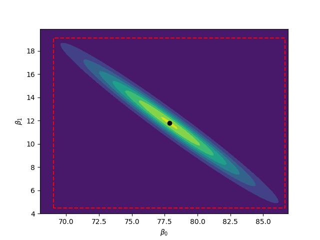
Since a priori I didn’t know anything about the process from which the data was taken, I used noninformative priors for the \(\beta\) and \(\sigma^2\). The next figure shows the posterior joint distribution of \(\beta_0\) and \(\beta_1\), which we know that follows a multivariate \(t\) distribution, I have added individual intervals of posteriori probability of 0.95 for each one. Note that there are a lot of points in the intervals, that are not likely at all when we consider the joint distribution.

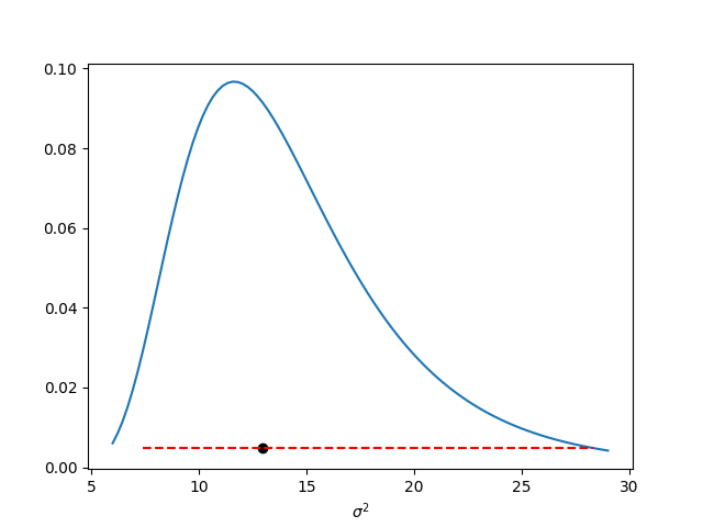
Similarly, in the next image I present the posterior distribution of \(\sigma^2\) with a posterior interval of probability 0.95 obtained with the quantiles method, i.e. the interval is given by the quantiles of probability 0.025 and 0.975.

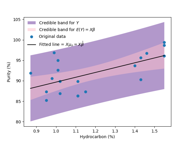
Finally, in the next image I present the scatterplot with the fitted regression line, I present posterior intervals for both, the regression function and observations comming from the process analyzed. It is common in the Bayesian framework to call them “Credible intervals”, other authors have proposed to call them “Compatibility intervals”.

5.3. Exercises

1. Verify the expressions for the normal inverse \(\chi^2\) model presentedn in Chapter 4 using the expressions given in this chapter.