4. Normal likelihood with mean and variance unknown

4.1. Normal likelihood with noninformative prior

Let be \(Y_1,\ldots,Y_n|\mu,\sigma^2\overset{iid}{\sim}\textsf{Normal}(\mu,\sigma^2)\), so the likelihood evaluated in our sample is given by

\[p(\mathbf{Y}|\mu,\sigma^2)=\frac{1}{(2\pi)^{n/2}\sigma^n}\exp\left\{-\frac{1}{2\sigma^2}\sum_{i=1}^n (y_i-\mu)^2\right\}.\]

In Chapter 6 we’ll see that, because \(\mu\) and \(\sigma\) are parameters of location and scale, respectively, then a noninformative prior is given by

\[p(\mu,\sigma^2)\propto \frac{1}{\sigma^2}1_{\mathbb{R}}(\mu)1_{(0,\infty)}(\sigma^2).\]

Thus,

\[\begin{split} \begin{align*} p(\mu,\sigma^2|\mathbf{Y}) &\propto \sigma^{-n-2}\exp\left\{-\frac{1}{2\sigma^2}\sum_{i=1}^n (y_i-\mu)^2\right\} \\\\ &= \sigma^{-n-2}\exp\left\{-\frac{1}{2\sigma^2}\left[\sum_{i=1}^n (y_i-\bar{y})^2+n(\bar{y}-\mu)^2\right]\right\} \\\\ &= \sigma^{-n-2}\exp\left\{-\frac{1}{2\sigma^2}\left[(n-1)s^2+n(\bar{y}-\mu)^2\right]\right\}, \end{align*} \end{split}\]

where

\[s^2=\frac{1}{n-1}\sum_{i=1}^n (y_i-\bar{y})^2.\]

4.1.1. Distribution of \(\mu|\sigma^2,\mathbf{Y}\)

From the previous expression we can deduce the distribution of \(\mu|\sigma^2,\mathbf{Y}\) taking \(\sigma^2\) as a constant,

\[p(\mu|\sigma^2,\mathbf{Y})\propto \exp\left\{-\frac{n}{2\sigma^2}(\bar{y}-\mu)^2\right\}.\]

That is,

\[\mu|\sigma^2,\mathbf{Y}\sim\textsf{Normal}(\bar{y},\sigma^2/n).\]

4.1.2. Distribution of \(\sigma^2|\mathbf{Y}\)

To get the distribution of \(\sigma^2|\mathbf{Y}\) we can marginalize \(p(\mu,\sigma^2|\mathbf{Y})\) with respect to \(\mu\). That is, we can calculate the next integral

\[\begin{split} \begin{align*} p(\sigma^2|\mathbf{Y}) &= \int p(\mu,\sigma^2|\mathbf{Y})d\mu \\\\ &\propto \int\sigma^{-n-2}\exp\left\{-\frac{1}{2\sigma^2}\left[(n-1)s^2+n(\bar{y}-\mu)^2\right]\right\}d\mu \\\\ &\propto \sigma^{-n-2}\exp\left\{-\frac{(n-1)s^2}{2\sigma^2}\right\}\int\exp\left\{-\frac{1}{2\sigma^2}\left[n(\bar{y}-\mu)^2\right]\right\}d\mu \\\\ &\propto (\sigma^2)^{-(n+1)/2}\exp\left\{-\frac{(n-1)s^2}{2\sigma^2}\right\}, \end{align*} \end{split}\]

which corresponds with a scaled inverse \(\chi^2\) with \(n-1\) degrees of freedom and scale parameter \(s^2\), that is

\[\sigma^2|\mathbf{Y}\sim\textsf{Inverse-}\chi^2(n-1,s^2).\]

4.1.3. Distribution of \(\mu|\mathbf{Y}\)

Analogously, we can obtain the distribution of \(\mu|\mathbf{Y}\) marginalizing the joint posterior, that is

\[\begin{split} \begin{align*} p(\mu|\mathbf{Y}) &= \int p(\mu,\sigma^2|\mathbf{Y})d\sigma^2 \\\\ &\propto \int\sigma^{-n-2}\exp\left\{-\frac{1}{2\sigma^2}\left[(n-1)s^2+n(\bar{y}-\mu)^2\right]\right\}d\sigma^2. \end{align*} \end{split}\]

This integral can be calculated making the change of variable

\[z=\frac{A}{2\sigma^2},\text{ donde }A=(n-1)s^2+n(\mu-\bar{y})^2.\]

Then,

\[\begin{split} \begin{align*} p(\mu|\mathbf{Y}) &\propto A^{-n/2}\int_0^\infty z^{(n-2)/2}\exp\{-z\}dz \\\\ &\propto \left[(n-1)s^2+n(\mu-\bar{y})^2\right]^{-n/2} \\\\ &\propto \left[1+\frac{n(\mu-\bar{y})^2}{(n-1)s^2}\right]^{-n/2}, \end{align*} \end{split}\]

which corresponds to the kernel of a \(t\) distribution with \(n-1\) degrees of freedom, with location parameter \(\bar{y}\) and scale parameter \(s/\sqrt{n}\). That is,

\[\mu|\mathbf{Y}\sim t_{n-1}(\bar{y}, s^2/n).\]

4.1.4. Connection with the frequentist statistics

In other words, considering noninformative priors for \(\mu\) and \(\sigma^2\), we have that

\[\sqrt{n}\frac{\mu-\bar{y}}{\sigma}\Big|\sigma^2,\mathbf{Y}\sim\textsf{Normal}(0,1).\]

Meanwhile, the central limit theorem stablishes that

\[\sqrt{n}\frac{\bar{y}-\mu}{\sigma}\Big|\mu,\sigma^2\sim\textsf{Normal}(0,1).\]

We also prove that

\[\sqrt{n}\frac{\mu-\bar{y}}{s}\Big|\mathbf{Y}\sim t_{n-1},\]

which coincides with the result of the frequentist statistics: $\(\sqrt{n}\frac{\bar{y}-\mu}{s}\Big|\mu\sim t_{n-1}.\)$

4.1.5. Simulate from the posterior predictive distribution

Once we obtained the posterior distributions, it is easy to simulate from the posterior predictive distribution, we just need to execute the following steps:

1. Simulate \(\tilde{\sigma}^2\sim\textsf{Inverse-}\chi^2(n-1,s^2).\)

2. Simulate \(\tilde{\mu}\sim\textsf{Normal}(\bar{y},\tilde{\sigma}^2/n)\).

3. Simulate \(\tilde{Y}\sim\textsf{Normal}(\tilde{\mu},\tilde{\sigma}^2)\).

4.2. Normal - Inverse-\(\chi^2\) prior for the normal likelihood

It is well-known that the prior Normal - Inverse-\(\chi^2\) forms a conjugate model for the normal likelihood. If

\[\begin{split} \begin{align*} \mu|\sigma^2 &\sim \textsf{Normal}(\mu_0,\sigma^2/\kappa_0) \\ \sigma^2 &\sim \textsf{Inverse-}\chi^2(\nu_0,\sigma_0^2) \end{align*} \end{split}\]

and \(Y_1,\ldots,Y_n|\mu,\sigma^2\overset{iid}{\sim}\textsf{Normal}(\mu,\sigma^2)\). Then,

\[\begin{split} \begin{align*} \mu|\sigma^2,\mathbf{Y} &\sim \textsf{Normal}(\mu_n,\sigma^2/\kappa_n)\\ \sigma^2|\mathbf{Y} &\sim \textsf{Inverse-}\chi^2(\nu_n,\sigma_n^2), \end{align*} \end{split}\]

where

\[\begin{split} \begin{align*} \mu_n &= \frac{\kappa_0}{\kappa_0+n}\mu_0 + \frac{n}{\kappa_0+n}\bar{y} \\ \kappa_n &= \kappa_0+n \\ \nu_n &= \nu_0+n \\ \nu_n\sigma_n^2 &= \nu_0\sigma_0^2+(n-1)s^2+\frac{\kappa_0 n}{\kappa_0+n}(\bar{y}-\mu_0)^2 \end{align*} \end{split}\]

and \(s^2=\frac{1}{n-1}\sum_{i=1}^n(y_i-\bar{y})^2\).

More over,

\[\mu|\mathbf{Y}\sim t_{\nu_n}(\mu_n, \sigma_n^2/\kappa_n)\]

and

\[Y|\mathbf{Y}\sim t_{\nu_n}\left(\mu_n, \frac{(1+\kappa_n)\sigma_n^2}{\kappa_n}\right).\]

4.3. Bayesian statistical process control

Because

\[Y|\mathbf{Y}\sim t_{\nu_n}\left(\mu_n, \frac{(1+\kappa_n)\sigma_n^2}{\kappa_n}\right),\]

then

\[\mathbb{E}[Y|\mathbf{Y}] = \mu_n\quad\text{and}\quad \mathbb{V}[Y|\mathbf{Y}]=\left(\frac{\nu_n}{\nu_n-2}\right)\left(\frac{1+\kappa_n}{\kappa_n}\right)\sigma_n^2.\]

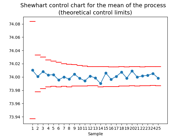
4.3.1. Control intervals for \(\bar{Y}\)

Let be

\[\bar{Y}_m=\frac{1}{m}\sum_{i=1}^m Y_i.\]

Thus, an approximate prediction interval of posterior probability \((1-\alpha)\times 100\%\) for the sample average \(\bar{Y}_m\) is given by

\[\mu_n \pm q_{t_{\nu_n}}(1-\alpha/2)\frac{1}{\sqrt{m}}\left(\frac{\nu_n}{\nu_n-2}\right)^{1/2}\left(\frac{1+\kappa_n}{\kappa_n}\right)^{1/2}\sigma_n,\]

where \(q_{t_{\nu_n}}(1-\alpha/2)\) denotes the quantile of probability \(1-\alpha/2\) of a \(t\) distribution with \(\nu_n\) degrees of freedom.

In the field of statistical process control, the extremes of the prediction interval are called lower and upper control limitis (LCL and UCL, respectively). It is usual to consider \(\alpha=0.002\), so the interval coincides with the normal case of \(\pm 3\sigma\).

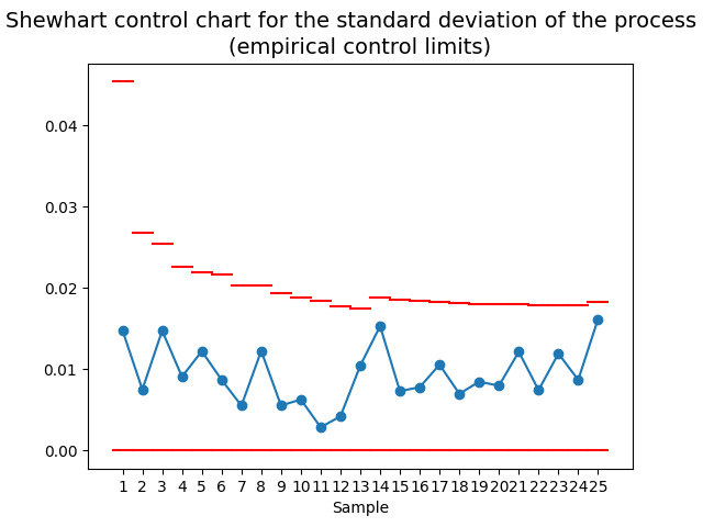
4.3.2. Control intervals for \(S\)

When monitoring a process, it’s important to check not only its mean but also the behavior of its variability. Unfortunately, it is not easy to find theoretical control limits for the sample deviaton \(S\). But not everything is lost, we can use simulation to solve the problem! We just need to perform the following steps:

1. Simulate \(J\) samples \(Y_1,\ldots,Y_n\) from the posterior predictive distribution, with \(J\) large.

2. The sample deviation of each one of the simulated samples, \(S_1,\ldots,S_J\) will follow the same distribution that the sample deviattion \(S\) of our original observations.

3. Using the sample \(S_1,\ldots,S_J\), we calculate its mean \(\bar{S}\) and standard deviation \(S_S\).

4. We can define the \(\pm 3\sigma\) control limits as

\[UCL=\bar{S} + 3 S_S\quad\text{y}\quad LCL=\max\{0, \bar{S} - 3 S_S\}.\]

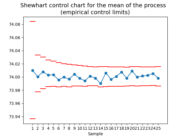
4.3.3. Simulated control intervals for \(\bar{Y}\)

Similarly, we can obtain a sample of the sample average \(\bar{Y}_1,\ldots,\bar{Y}_J\) and estimate its control limits as:

\[UCL=\bar{\bar{Y}} + q_{t_{\nu_n}}(1-\alpha/2) S_{\bar{Y}}\quad\text{and}\quad LCL=\bar{\bar{Y}} - q_{t_{\nu_n}}(1-\alpha/2) S_{\bar{Y}}.\]

4.3.4. Setting the hyperparameters

Because a priori we know nothing about the process, we can use the reference prior given by

\[p(\mu,\sigma^2)\propto\frac{1}{\sigma^2}1_{\mathbb{R}}(\mu)1_{(0,\infty)}(\sigma^2),\]

which is obtained setting the hyperparameters in the following values:

\[\kappa_0=0,\quad \mu_0\in\mathbb{R},\quad\nu_0=-1,\quad\sigma_0^2=0.\]

4.3.5. Example

Note

The data for this example were taken from Table 6.3 of [Mon19], seventh edition.

Shewhart control charts

Different control charts have been proposed for different purposes. The type of control charts presented here are known as Shewhart control charts.

See also

For interested readers in the field of Statistical Quality Control, of which control charts form part, I recomend the book [Mon19].

4.4. Predictive distribution of the normal likelihood with unknown variance

Back in Chapter 3 we study the case where our data comes from a normal distribution with unknown variance. We found that the conjugate distribution in such case is an scaled inverse \(\chi^2\) distribution, we are now ready to deduce its posterior predictive distribution.

Consider the posterior distributions of the Normal - Inverse-\(\chi^2\) prior for the normal likelihood,

\[\begin{split} \begin{align*} \mu|\sigma^2,\mathbf{Y} &\sim \textsf{Normal}(\mu_n,\sigma^2/\kappa_n) \\ \sigma^2|\mathbf{Y} &\sim \textsf{Inverse-}\chi^2(\nu_n,\sigma_n^2) \end{align*} \end{split}\]

and

\[\mu|\mathbf{Y}\sim t_{\nu_n}(\mu_n,\sigma_n^2/\kappa_n).\]

Note that

\[\begin{split} \begin{align*} p(\mu|\mathbf{Y}) & = \int p(\mu,\sigma^2|\mathbf{Y})d\sigma^2 \\ & = \int p(\mu|\sigma^2,\mathbf{Y})p(\sigma^2|\mathbf{Y})d\sigma^2. \end{align*} \end{split}\]

That is,

\[t_{\nu_n}(\mu_n,\sigma_n^2/\kappa_n) = \int\textsf{Normal}(\mu_n,\sigma^2/\kappa_n)\textsf{Inverse-}\chi^2(\nu_n,\sigma_n^2)d\sigma^2.\]

On the other hand, consider the model with \(\mu\) known but \(\sigma^2\) unknown,

\[\begin{split} \begin{align*} Y|\sigma^2 & \sim \textsf{Normal}(\mu,\sigma^2) \\ \sigma^2 & \sim \textsf{Inverse-}\chi^2(\nu_0,\sigma_0^2), \end{align*} \end{split}\]

then

\[\sigma^2|\mathbf{Y}\sim\textsf{Inverse-}\chi^2(\nu_n,\sigma_n^2),\]

where

\[\nu_n=\nu_0+n,\quad \sigma_n^2=\frac{\nu_0\sigma_0^2+nv}{\nu_0+n}\]

and

\[v=\frac{1}{n}\sum_{i=1}^n (Y_i-\mu)^2.\]

Note that

\[\begin{split} \begin{align*} p(Y|\mathbf{Y}) & = \int p(Y,\sigma^2|\mathbf{Y})d\sigma^2 \\ & = \int p(Y|\sigma^2,\mathbf{Y})p(\sigma^2|\mathbf{Y})d\sigma^2 \\ & = \int \textsf{Normal}(\mu,\sigma^2)\textsf{Inverse-}\chi^2(\nu_n,\sigma_n^2)d\sigma^2, \end{align*} \end{split}\]

by analogy, we deduce that

\[Y|\mathbf{Y}\sim t_{\nu_n}(\mu,\sigma_n^2).\]

Furthermore, in this case the noninformative prior is acgieved setting \(\nu_0=0\) and \(\sigma_0^2>0\), so \(\nu_n=n\) and \(\sigma_n^2=v\). Then,

\[Y|\mathbf{Y}\sim t_n(\mu,v),\]

or, equivalently

\[\frac{Y-\mu}{\sqrt{v}}|\mathbf{Y}\sim t_n.\]

4.5. Exercises